Pandas Introduction#

Pandas is an open-source library for data analysis and data processing, based on the Python programming language.

Pandas provides easy-to-use data structures and data analysis tools, especially suitable for handling structured data such as tabular data (similar to Excel spreadsheets).

Pandas is one of the commonly used tools in data science and analytics, enabling users to easily import data from various data sources and perform efficient operations and analysis on the data.

Pandas introduces two main data structures: DataFrame and Series

• Series: Similar to a one-dimensional array or list, consisting of a set of data and associated data labels (indices). A Series can be viewed as a column in a DataFrame, or as a standalone one-dimensional data structure.
• DataFrame: Similar to a two-dimensional table, it is the most important data structure in Pandas. DataFrame can be seen as a table composed of multiple Series arranged by column; it has both row indices and column indices, making it convenient to perform row/column selection, filtering, merging, etc.

Pandas provides a rich set of features, including:

• Data cleaning: handling missing data, duplicate data, etc.
• Data transformation: changing the shape, structure, or format of data.
• Data analysis: performing statistical analysis, aggregation, grouping, etc.
• Data visualization: by integrating libraries such as Matplotlib and Seaborn, you can perform data visualization.

Pandas Installation#

1. Install Python

   Download from the official site / Docker installation

2. Install Pandas

   pip install pandas

   Validation:

   1
   import pandas as pd
   2
   pd.__version__

Structure#

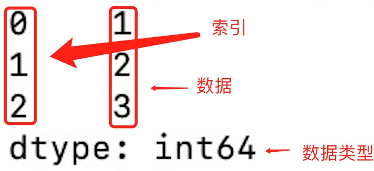
• Index: Each Series has an index, which can be integers, strings, dates, etc. If no explicit index is specified, Pandas automatically creates a default integer index.
• Data type: A Series can contain elements of different data types, including integers, floats, strings, etc.

1
pandas.Series( data, index, dtype, name, copy)
2

3
## data：A set of data (ndarray type).
4
## index：Data indexing labels; if not specified, default starts from 0.
5
## dtype：Data type; defaults to auto-detection.
6
## name：Set the name.
7
## copy：Copy the data, defaults to False.

Examples#

1. Using series

   1
   import pandas as pd
   2
   
   3
   a = [1, 2, 3]
   4
   myvar = pd.Series(a)
   5
   print(myvar)
   6
   print(myvar[1])

   Output:

   

2. Setting index with pd.Series

   1
   import pandas as pd
   2
   
   3
   a = ["Google", "Runoob", "Wiki"]
   4
   myvar = pd.Series(a, index = ["x", "y", "z"])
   5
   print(myvar)
   6
   print(myvar["y"])

3. Creating from a dictionary

   1
   import pandas as pd
   2
   
   3
   sites = {1: "Google", 2: "Runoob", 3: "Wiki"}
   4
   myvar = pd.Series(sites)
   5
   print(myvar)
   6
   
   7
   myvar = pd.Series(sites, index = [1, 2], name="RUNOOB-Series-TEST" )
   8
   print(myvar)
   9
   
   10
   myvar = pd.Series(sites, index = [1, 2], name="RUNOOB-Series-TEST" )
   11
   print(myvar)

Basic Operations#

• Basic Operations

  1
  ## Get value
  2
  value = series[2]  ## Get the value with index 2
  3
  
  4
  ## Get multiple values
  5
  subset = series[1:4]  ## Get the values with index 1 to 3
  6
  
  7
  ## Use a custom index
  8
  value = series_with_index['b']  ## Get the value for index 'b'
  9
  
  10
  ## Index and value correspondence
  11
  for index, value in series_with_index.items():
  12
      print(f"Index: {index}, Value: {value}")

• Arithmetic Operations

  1
  ## Arithmetic operations
  2
  result = series * 2  ## Multiply all elements by 2
  3
  
  4
  ## Filtering
  5
  filtered_series = series[series > 2]  ## Select elements greater than 2
  6
  
  7
  ## Mathematical functions
  8
  import numpy as np
  9
  result = np.sqrt(series)  ## Take the square root of each element

• Attributes and Methods

  1
  ## Get index
  2
  index = series_with_index.index
  3
  
  4
  ## Get values array
  5
  values = series_with_index.values
  6
  
  7
  ## Get descriptive statistics
  8
  stats = series_with_index.describe()
  9
  
  10
  ## Get the index of the maximum and minimum values
  11
  max_index = series_with_index.idxmax()
  12
  min_index = series_with_index.idxmin()

• Notes

  • Data in a Series is ordered.
  • A Series can be viewed as a one-dimensional array with an index.
  • The index can be unique, but it is not required.
  • Data can be scalars, lists, NumPy arrays, etc.

DataFrame Structure#

• Columns and rows: DataFrame is composed of multiple columns, each column has a name and can be seen as a Series. At the same time, DataFrame has a row index used to identify each row.
• Two-dimensional structure: DataFrame is a two-dimensional table with rows and columns. It can be viewed as a dictionary of multiple Series objects.
• Data types of columns: Different columns can contain different data types, such as integers, floats, strings, etc.

1
pandas.DataFrame( data, index, columns, dtype, copy)
2

3
# data：A set of data (ndarray, series, map, lists, dict types).
4
# index: The index values, or row labels
5
# columns: Column labels, default is RangeIndex (0, 1, 2, ..., n)
6
# dtype: Data type; defaults to auto-detection.
7
# copy: Copy the data, defaults to False.

DataFrame Examples#

1. Using DataFrame

   1
   import pandas as pd
   2
   
   3
   data = [['Google',10],['Runoob',12],['Wiki',13]]
   4
   df = pd.DataFrame(data,columns=['Site','Age'])
   5
   print(df)

2. Creating from ndarrays

   1
   import pandas as pd
   2
   
   3
   data = {'Site':['Google', 'Runoob', 'Wiki'], 'Age':[10, 12, 13]}
   4
   df = pd.DataFrame(data)
   5
   print (df)

3. Creating from dictionaries

   1
   import pandas as pd
   2
   
   3
   data = [{'a': 1, 'b': 2},{'a': 5, 'b': 10, 'c': 20}]
   4
   df = pd.DataFrame(data)
   5
   print (df)

   Missing parts of data are NaN.

4. Returning specified rows with loc Pandas can use the loc attribute to return data for specified rows. If no index is set, the first row has index 0, the second row 1, and so on

   1
   import pandas as pd
   2
   
   3
   data = {
   4
     "calories": [420, 380, 390],
   5
     "duration": [50, 40, 45]
   6
   }
   7
   
   8
   # Load data into a DataFrame object
   9
   df = pd.DataFrame(data)
   10
   
   11
   # Return the first row
   12
   print(df.loc[0])
   13
   # Return the second row
   14
   print(df.loc[1])
   15
   
   16
   # Return the first and second rows
   17
   print(df.loc[[0, 1]])
   18
   
   19
   # Specify the index
   20
   print(df.loc["duration"])

5. pd.DataFrame with specified index

   1
   import pandas as pd
   2
   data = {
   3
     "calories": [420, 380, 390],
   4
     "duration": [50, 40, 45]
   5
   }
   6
   
   7
   df = pd.DataFrame(data, index = ["day1", "day2", "day3"])
   8
   print(df)

Basic DataFrame Operations#

• Basic Operations

  1
  # Get a column
  2
  name_column = df['Name']
  3
  
  4
  # Get a row
  5
  first_row = df.loc[0]
  6
  
  7
  # Select multiple columns
  8
  subset = df[['Name', 'Age']]
  9
  
  10
  # Filter rows
  11
  filtered_rows = df[df['Age'] > 30]

• Data Manipulation

  1
  # Add a new column
  2
  df['Salary'] = [50000, 60000, 70000]
  3
  
  4
  # Delete a column
  5
  df.drop('City', axis=1, inplace=True)
  6
  
  7
  # Sort
  8
  df.sort_values(by='Age', ascending=False, inplace=True)
  9
  
  10
  # Rename a column
  11
  df.rename(columns={'Name': 'Full Name'}, inplace=True)

• Attributes and Methods

  1
  # Get column names
  2
  columns = df.columns
  3
  
  4
  # Get shape (rows and columns)
  5
  shape = df.shape
  6
  
  7
  # Get index
  8
  index = df.index
  9
  
  10
  # Get descriptive statistics
  11
  stats = df.describe()

• Creating from external data sources

  1
  # Create DataFrame from a CSV file
  2
  df_csv = pd.read_csv('example.csv')
  3
  
  4
  # Create DataFrame from an Excel file
  5
  df_excel = pd.read_excel('example.xlsx')
  6
  
  7
  # Create DataFrame from a list of dictionaries
  8
  data_list = [{'Name': 'Alice', 'Age': 25}, {'Name': 'Bob', 'Age': 30}]
  9
  df_from_list = pd.DataFrame(data_list)

• Notes

  • DataFrame is a flexible data structure that can accommodate columns with different data types.
  • Column names and row indices can be strings, integers, etc.
  • DataFrame can be queried, filtered, modified, and analyzed in many ways.
  • Through working with DataFrame, you can perform data cleaning, transformation, analysis, and visualization.

Introduction#

CSV (Comma-Separated Values; sometimes also referred to as Character-Separated Values, since the separator character can be something other than a comma) stores tabular data (numbers and text) in plain text files.

CSV is a general-purpose, relatively simple file format widely used by users, businesses, and scientists.

1. Handling CSVs Pandas can easily handle CSV files

   1
   import pandas as pd
   2
   df = pd.read_csv('site.csv')
   3
   print(df.to_string())

2. Storing CSVs You can use the to_csv() method to store a DataFrame as a CSV file

   1
   import pandas as pd
   2
   
   3
   # Three fields name, site, age
   4
   nme = ["Google", "Runoob", "Taobao", "Wiki"]
   5
   st = ["www.google.com", "www.runoob.com", "www.taobao.com", "www.wikipedia.org"]
   6
   ag = [90, 40, 80, 98]
   7
   # Dictionary
   8
   dict = {'name': nme, 'site': st, 'age': ag}
   9
   df = pd.DataFrame(dict)
   10
   
   11
   # Save dataframe
   12
   df.to_csv('site.csv')

Data Processing#

1
import pandas as pd
2

3
df = pd.read_csv('nba.csv')
4
print(df.head())
5

6
print(df.head(10))

1
import pandas as pd
2

3
df = pd.read_csv('nba.csv')
4
print(df.tail())
5

6
print(df.tail(10))

1
import pandas as pd
2

3
df = pd.read_csv('nba.csv')
4
print(df.info())

Plain JSON Handling#

1
import pandas as pd
2

3
df = pd.read_json('sites.json')
4
print(df.to_string())
5

6
URL = '<https://static.runoob.com/download/sites.json>'
7
df = pd.read_json(URL)
8
print(df)

JSON objects have the same format as Python dictionaries, so we can directly convert Python dictionaries into DataFrame data

Nested JSON Handling#

Using the json_normalize() method to fully parse nested data

1
import pandas as pd
2
import json
3

4
# Load data using Python's JSON module
5
with open('nested_list.json','r') as f:
6
    data = json.loads(f.read())
7

8
# Flatten data
9
df_nested_list = pd.json_normalize(data, record_path =['students'])
10
print(df_nested_list)

More complex data

1
import pandas as pd
2
import json
3

4
# Load data using Python's JSON module
5
with open('nested_mix.json','r') as f:
6
    data = json.loads(f.read())
7

8
df = pd.json_normalize(
9
    data,
10
    record_path =['students'],
11
    meta=[
12
        'class',
13
        ['info', 'president'],
14
        ['info', 'contacts', 'tel']
15
    ]
16
)
17

18
print(df)

Reading a Group of Data from Nested JSON#

Use the glom module to handle nested data; the glom module allows us to access nested object attributes using dot notation

• Install glom

  1
  pip3 install glom

• Usage

  1
  import pandas as pd
  2
  from glom import glom
  3
  
  4
  df = pd.read_json('nested_deep.json')
  5
  
  6
  data = df['students'].apply(lambda row: glom(row, 'grade.math'))
  7
  print(data)

Cleaning Missing Values#

If we want to delete rows that contain empty fields, we can use the dropna() method; the syntax is as follows:

1
DataFrame.dropna(axis=0, how='any', thresh=None, subset=None, inplace=False)
2

3
# axis: defaults to 0, meaning drop the entire row when a missing value is present; if axis=1 is set, drop the entire column.
4
# how: defaults to 'any'. If any data in a row (or column) has NA, drop the entire row; if how='all', a row (or column) where all values are NA is dropped.
5
# thresh: set how many non-empty values are required to keep the row.
6
# subset: set the columns to check. If multiple columns, you can use a list of column names.
7
# inplace: If True is set, the calculated values overwrite the previous values and return None, modifying the source data.

You can use isnull() to determine whether each cell is empty.

In pandas.read_csv you can specify na_values to designate missing values

1
import pandas as pd
2

3
df = pd.read_csv('property-data.csv')
4

5
print(df['NUM_BEDROOMS'])
6
print(df['NUM_BEDROOMS'].isnull())
7

8
# Specify missing data
9
missing_values = ["n/a", "na", "--"]
10
df = pd.read_csv('property-data.csv', na_values = missing_values)
11

12
print (df['NUM_BEDROOMS'])
13
print (df['NUM_BEDROOMS'].isnull())
14

15
# Remove missing data
16
new_df = df.dropna()
17
print(new_df.to_string())
18

19
# Modify the original DataFrame
20
df.dropna(inplace = True)
21
print(df.to_string())
22

23
# Remove rows with missing values in specified columns
24
df.dropna(subset=['ST_NUM'], inplace = True)
25
print(df.to_string())

Using fillna() to replace missing values

A common method to replace empty cells is to compute the mean, median, or mode of the column.

Pandas uses mean(), median(), and mode() to compute the column mean (the average of all values), median (the middle value after sorting), and mode (the value that appears most frequently).

1
import pandas as pd
2

3
df = pd.read_csv('property-data.csv')
4

5
# Replace missing fields with 12345
6
df.fillna(12345, inplace = True)
7
print(df.to_string())
8

9
# Replace missing fields with the mean
10
x = df["ST_NUM"].mean()
11
df["ST_NUM"].fillna(x, inplace = True)
12
print(df.to_string())
13

14
# Replace missing fields with the median
15
x = df["ST_NUM"].median()
16
df["ST_NUM"].fillna(x, inplace = True)
17
print(df.to_string())
18

19
# Replace missing fields with the mode
20
x = df["ST_NUM"].mode()
21
df["ST_NUM"].fillna(x, inplace = True)
22
print(df.to_string())

Cleaning Incorrect Data#

Data with incorrect formats can make data analysis difficult, even impossible.

We can address this by either including rows with empty cells, or converting all cells in a column to the same format data.

1
import pandas as pd
2

3
# The third date format is incorrect
4
data = {
5
  "Date": ['2020/12/01', '2020/12/02' , '20201226'],
6
  "duration": [50, 40, 45]
7
}
8
df = pd.DataFrame(data, index = ["day1", "day2", "day3"])
9

10
# In newer Python 3, the following will raise an error; you need to specify format='mixed' to clearly indicate mixed formats to run properly
11
# pd.to_datetime(df['Date'])
12
df['Date'] = pd.to_datetime(df['Date'], format='mixed')
13
print(df.to_string())

Using astype to modify data types

1
data['语文'].dropna(how='any').astype('int')

Cleaning Erroneous Data#

1
import pandas as pd
2

3
person = {
4
  "name": ['Google', 'Runoob' , 'Taobao'],
5
  "age": [50, 200, 12345]
6
}
7

8
df = pd.DataFrame(person)
9

10
# Directly modify data
11
df.loc[2, 'age'] = 30
12

13
# Loop-based checks
14
for x in df.index:
15
  if df.loc[x, "age"] > 120:
16
    df.loc[x, "age"] = 120
17

18
# Delete rows
19
for x in df.index:
20
  if df.loc[x, "age"] > 120:
21
    df.drop(x, inplace = True)
22

23
print(df.to_string())

1
import pandas as pd
2

3
person = {
4
  "name": ['Google', 'Runoob', 'Runoob', 'Taobao'],
5
  "age": [50, 40, 40, 23]
6
}
7
df = pd.DataFrame(person)
8

9
# Find duplicated data
10
print(df.duplicated())
11

12
# Remove duplicate data
13
df.drop_duplicates(inplace = True)
14
print(df)